2016 October 27,
This assignment is a sequence is disconnected exercises, intended to help you learn recursion. In each exercise, your function should call itself to do its work. You should not need to write or use any other helper functions. You may complete this assignment individually, or with one partner. Submit your work electronically, by Wednesday at the start of class.
Recall from one of our early tutorials that Paul's monologue length is the number of integers that Paul speaks, when started with a given integer. For example, the monologue length of 5 is 6, because Paul says "5, 16, 8, 4, 2, 1" when started with the number 5. Write the following function recursively.
# Computes Paul's monologue length.
# Input: Positive integer n.
# Returns: Positive integer.
def monologueLength(n):
In mathematics, the combination function choose(n, k) computes how many ways there are to choose k objects from a set of n objects. For example, choose(4, 2) is 6, because there are six ways to choose two objects from a set of four objects. (If the four objects are called A, B, C, and D, then we can choose A and B, A and C, A and D, B and C, B and D, or C and D.) There are a couple of trivial cases: choose(n, 0) is defined to be 1, and choose(n, n) is also defined to be 1.
It turns out that choose is related to factorials like this: choose(n, k) equals n! / (k! (n - k)!). Thus, we could implement choose using a factorial function, which we already have. However, factorials get big extremely rapidly. Python can handle large numbers pretty easily, but many programming languages can't, so it's good to have a way of computing choose that doesn't use factorials.
Here's another handy property of the choose function: choose(n, k) equals choose(n - 1, k) + choose(n - 1, k - 1). Use this property to implement the choose function recursively, without any factorials.
# Computes the combination function n! / (k! (n - k)!).
# Input: Nonnegative integer n. Integer k such that 0 <= k <= n.
# Returns: Positive integer.
def choose(n, k):
In this exercise, you will write a function that draws a "dragon" fractal recursively. Its inputs are of the same kinds, playing the same roles, as in our drawKoch function.
# Draws a dragon fractal.
# Inputs: turtle. Float. Nonnegative integer.
# Returns: None.
def drawDragon(t, length, detail):
Here is the dragon fractal for length 200 and detail 0, 1, 2, 3, 4, 5:
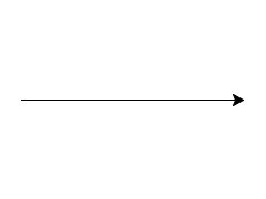

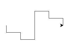
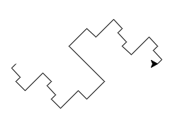
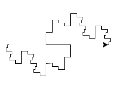
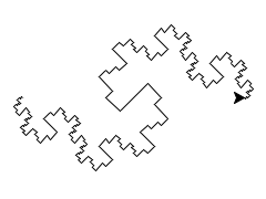
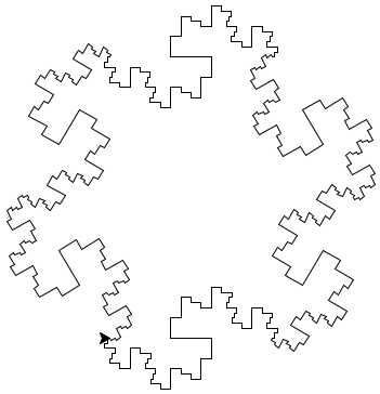
By the way, when people draw this kind of fractal, they usually join multiple copies together to form a closed curve. In the following example, I joined six copies. It may surprise you to learn that this shape perfectly interlocks with itself. If you were to make clay tiles in this shape, then you could tile your floor with them. (No, you are not required to make this image for this assignment.)
We've already done exercises like this one a couple of times in this course. This time we're doing it recursively. (But really this exercise is a warm-up for the next exercise, arraySum.)
# Computes the sum of two lists of numbers (of equal length >= 0).
# If the lists are empty, then returns the empty list.
# Input: List of numbers. List of numbers of the same length.
# Returns: List of numbers of the same length.
def listSum(a, b):
An array of numbers is a rectangular grid of numbers, of some dimension. Let me explain, through some examples:
But arrays don't stop there. Here's a 3 x 2 x 3 grid — that is, a (3, 2, 3)-array:
[[[0, 1, 1], [1, -1, 4]], [[2, 1, 2], [3, 3, 1]], [[-5, -1, 3], [2, 2, 2]]]
By now you can probably see where I'm going: For any k integers n1, n2, ..., nk ≥ 1, an (n1, n2, ..., nk)-array is an n1 x n2 x ... x nk grid of numbers. Whenever you have two arrays of the same dimensions (n1, n2, ..., nk), you can add them entry-by-entry to get a new (n1, n2, ..., nk)-array. For example, here are two (1, 3, 2, 3)-arrays, and their sum, which is also a (1, 3, 2, 3)-array:
> > > first = [[[[0, 1, 1], [1, -1, 4]], [[2, 1, 2], [3, 3, 1]], [[-5, -1, 3], [2, 2, 2]]]]
[[[[0, 1, 1], [1, -1, 4]], [[2, 1, 2], [3, 3, 1]], [[-5, -1, 3], [2, 2, 2]]]]
> > > second = [[[[5, 2, 2], [1, -1, 7]], [[2, 0, 0], [3, 9, 4]], [[4, 4, 4], [2, 2, 2]]]]
[[[[5, 2, 2], [1, -1, 7]], [[2, 0, 0], [3, 9, 4]], [[4, 4, 4], [2, 2, 2]]]]
> > > arraySum(first, second)
[[[[5, 3, 3], [2, -2, 11]], [[4, 1, 2], [6, 12, 5]], [[-1, 3, 7], [4, 4, 4]]]]
So your job is to implement this function recursively:
# Computes the sum of two arrays of numbers.
# Input: Array of numbers. Array of numbers of the same dimensions.
# Returns: Array of numbers of the same dimensions.
def arraySum(a, b):
Submit your work electronically. The grader will import your code into her/his own grading program and invoke your versions of the functions. They will be graded according to these criteria:
The rest of this assignment is optional. In algebra.py I have begun to implement a computer algebra system — software for performing algebraic calculations on complicated mathematical expressions. The code in algebra.py is heavily recursive, so it may help you study recursion. However, I did not write it recursively to be educational. I wrote it recursively because recursion is the natural way to write this kind of code.
As it's currently written, the software has one missing feature. You can't enter algebraic expressions such as "x * 4" in the usual syntax. Instead you have to use prefix syntax, which looks like "* x 4". And you enter the expression as a list. Once your expression is entered, you can use the beauty function to print it in the usual syntax. Here are two examples. (By the way, ^ denotes a power. It is more common than Python's ** notation.)
>>> f = ['*', 'x', 4]
>>> beauty(f)
'(x * 4)'
>>> g = ['sin', ['+', 7, 'x', ['^', 'x', 3]]]
>>> beauty(g)
'sin(7 + x + (x ^ 3))'
In the following example, we add the two expressions from the previous example.
>>> h = ['+', f, g]
>>> h
['+', ['*', 'x', 4], ['sin', ['+', 7, 'x', ['^', 'x', 3]]]]
>>> beauty(h)
'((x * 4) + sin(7 + x + (x ^ 3)))'
Here's how you evaluate a function (such as h) for a particular value (2) of a variable (x). Notice that value plugs in the value but doesn't do any further computation. Each part of my computer algebra system does its intended job and nothing else.
>>> hOf2 = value(h, 'x', 2)
>>> hOf2
['+', ['*', 2.0, 4.0], ['sin', ['+', 7.0, 2.0, ['^', 2.0, 3.0]]]]
>>> beauty(hOf2)
'((2.0 * 4.0) + sin(7.0 + 2.0 + (2.0 ^ 3.0)))'
To get the value as a number, simplify the preceding expression.
>>> simplification(hOf2)
7.0386025081204435
In general, algebraic simplification is quite a complicated process. Most of the code in algebra.py is devoted to simplification, and it can do much more than what we've seen so far, but it's still missing lots of features. If you're looking for something to do (other than the differentiation exercise below) then you might try to improve simplification.
This exercise asks you to add one feature to the computer algebra system: differentiation of functions. Differentiation is a topic from calculus. In principle I tell you everything you need to know below, but in practice you might find the exercise frustrating if you've never studied derivatives.
In math notation, the derivative of a function f with respect to a variable x can be denoted Dx f. Here are some rules of differentiation, in that notation. Notice that they are almost all recursive.
Your assignment is to add the following function to algebra.py.
def derivative(expr, var):
    """Given an expression and a string, regards the string as a variable name, differentiates the expression with respect to the variable, and returns the derivative as an expression."""
Here's a transcript demonstrating that my implementation works.
>>> h
['+', ['*', 'x', 4], ['sin', ['+', 7, 'x', ['^', 'x', 3]]]]
>>> beauty(h)
'((x * 4) + sin(7 + x + (x ^ 3)))'
>>> derivative(h, 'x')
['+', ['+', ['*', 1.0, 4], ['*', 'x', 0.0]], ['*', ['cos', ['+', 7, 'x', ['^', 'x', 3]]], ['+', 0.0, 1.0, ['*', 3, ['^', 'x', ['-', 3, 1.0]]]]]]
>>> simplification(derivative(h, 'x'))
['+', 4.0, ['*', ['cos', ['+', 7.0, 'x', ['^', 'x', 3.0]]], ['+', 1.0, ['*', 3.0, ['^', 'x', 2.0]]]]]
>>> beauty(simplification(derivative(h, 'x')))
'(4.0 + (cos(7.0 + x + (x ^ 3.0)) * (1.0 + (3.0 * (x ^ 2.0)))))'