2019 March 11,
You are not responsible for this material on any exam. I put it here, just to give you a glimpse of graphics topics that we didn't have time to explore.
A scene graph is a graph (network) that describes a scene. For example, a basic scene graph might be a tree of bodies connected in parent-child relationships. Typically each body is positioned and oriented relative to its parent. That is, its own isometry is multiplied by the isometries of its ancestors to produce the isometry that transforms it at run time. This structure allows bodies to be grouped so that they move cohesively together — like the body parts of a single human figure.
More sophisticated scene graphs can have other kinds of nodes. For example, a node might encode a switch to a different shader program. Another kind of node can implement level of detail (LoD). An LoD node has multiple children, all representing the same subscene at differing levels of detail. When the LoD node is told to render, it passes the message onto just one, or even none, of its children according to some criterion. For example, if the subscene is off-screen, it might be pruned entirely; but if it casts shadows onto the screen, then a low-detail version of it might be rendered in the first shadow-mapping pass.
Physics engines, which handle things such as gravity and collisions, often introduce their own graphs to model the relationships among bodies. My personal favorite, just because it is so accessible, is Open Dynamics Engine. In ODE, bodies can be connected by various kinds of joints: ball, hinge, etc. Joints are also made dynamically, whenever bodies collide or slide against each other. Here is a video demonstrating some of ODE's capabilities.
The next thing, that we were going to do in the course, is ray trace triangular meshes. Essentially, you loop over the triangles, testing intersection with each one. The problem is that there are many triangles. The image below is just the rocky part of the landscape that we rendered at hundreds of frames/second in OpenGL. In ray tracing it's more like hundreds of seconds per frame.
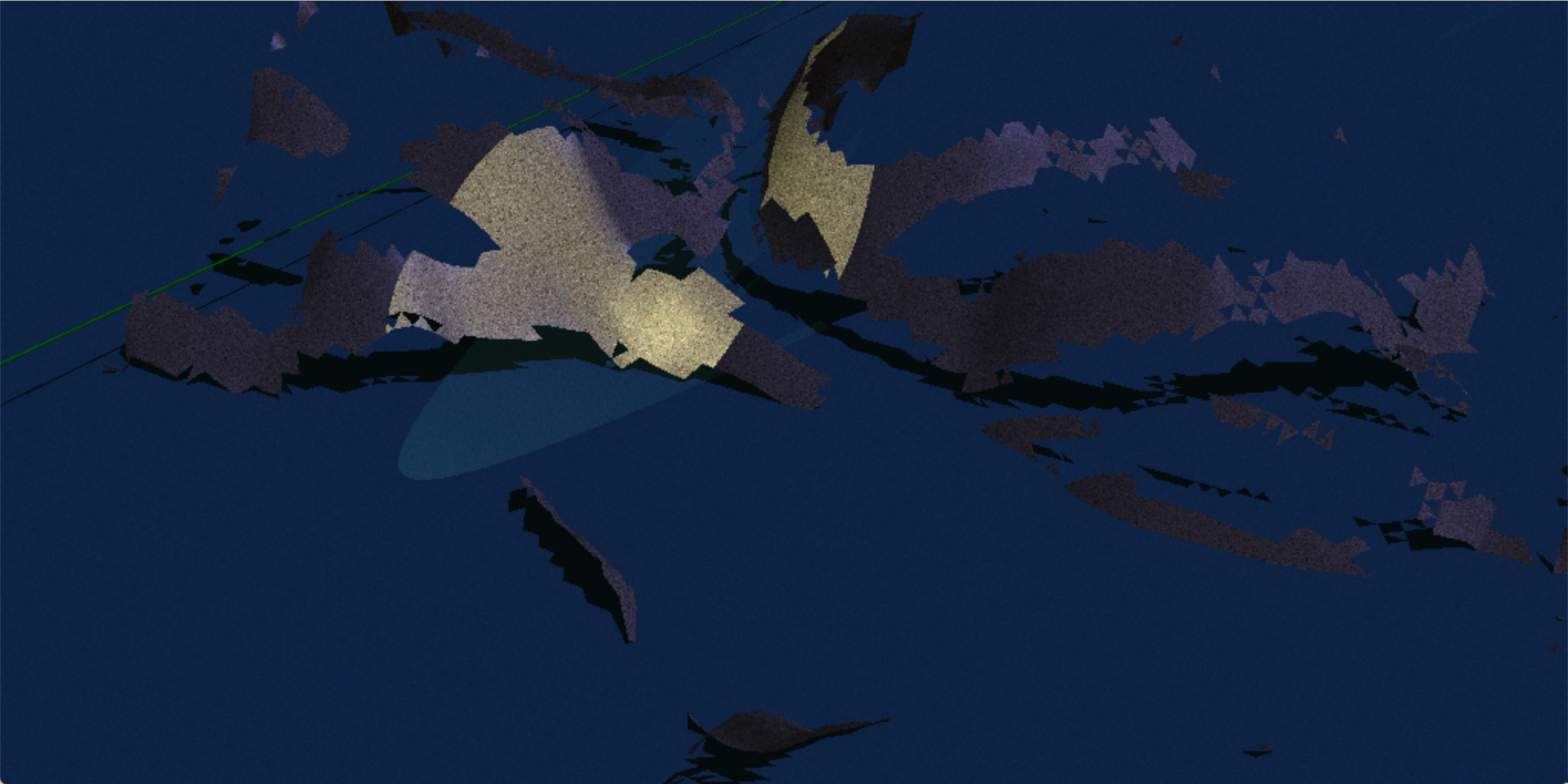
So a big part of ray tracing is designing data structures that speed up the intersection queries. Essentially, you enclose your meshes in simple primitives — spheres, axis-aligned boxes, etc. — for which intersections are fast. When testing intersection with a mesh, you first test intersection with the enclosing primitive; if there is no intersection, then you skip the mesh entirely. In fact, you probably want a hierarchy of enclosing primitives, which ends up looking a lot like a scene graph.
Ray tracing is highly parallelizable. So another way to improve the speed of ray tracing is to make it multi-threaded.
As far as improving the quality goes, the obvious next step is distribution ray tracing. This technique lets us soften our images in various ways — antialiasing, soft shadows (penumbras), blurry reflections, etc. — so that they appear less harsh and more natural. Here's the basic idea. Wherever we would cast a single ray in basic ray tracing, we instead cast multiple rays sampled from some probability distribution. Then we average the results of those rays. Yes, this is slow.
As of late 2018 and early 2019, video games are starting to augment their rasterizing engines with ray tracing. They get noticeably better lighting effects in certain situations, at the cost of other performance and quality compromises. For example, here is a detailed review of the graphics in Battlefield V. Check out the aggressive LoD culling on the ground around 11:55.
In our software rasterizing engine, we implemented nearest-neighbor texture filtering, linear texture filtering, and perspective-corrected interpolation. However, our textures still looked pretty poor. One reason is that good textures require careful artistic attention, which is outside the scope of this course. But there are also improved computational techniques, which we could have studied.
One such technique is mipmapping, in which the texture is prefiltered to several sizes. At run time, the size that best matches the screen size is automatically selected, so that minification and magnification are kept close to 1. The results are prettier than ours, with very little performance penalty. Another technique is anisotropic filtering, which incorporates perspective effects into the texture filtering itself. More generally, texture filtering is affected by large swathes of the theory of image processing.
Beyond texture mapping and shadow mapping, we mentioned several other mapping techniques, but we didn't have the time to implement them. One is mirror reflections off planar surfaces. Another is shadow mapping an omnidirectional light into a cube map. Another is shadow mapping a directional light. It's actually quite tricky, because the shadow viewing volume might need to be gigantic — encompassing the light, the regular viewing volume, and all space between them. A huge shadow viewing volume might require a high-resolution shadow map and a slow rendering pass to account for all of the shadow-casting bodies. This is a good time to use level-of-detail optimizations.
A mapping technique that we haven't mentioned is textured light. It can be used to model light passing through stained glass, for example. Based on your knowledge of shadow mapping, try to guess how it works. And there's lightmaps.
I've mentioned attenuation: the idea that light intensity should decrease with distance from the light source. I've mentioned ambient occlusion: the idea that fragments in crevices and corners should receive less ambient light. One effect I haven't mentioned is bloom. Also, we've used only the Phong lighting model, but there are others.
Radiosity is an approach to graphics that is different from both rasterization and ray tracing. The radiosity algorithm subdivides the scene into pieces, constructs linear equations governing how much light is bouncing between each pair of pieces, and solves the resulting linear system. This method can compute diffuse inter-reflection, which is difficult even for ray tracing.
Our mesh data structure is quite simple: a list of vertices and a list of triangles, with each triangle being three indices into the vertex list. However, many graphics applications endow meshes with more information. For example, each triangle might store three more integers: the indices of its three neighbor triangles. Such topological (connectivity) information enables various techniques. For example, a graphical mesh editing application might let the user pull on parts of the mesh, adjusting many interconnected triangles at once. For another example, if the mesh is a landscape, and we want AIs to traverse that landscape, then topological information helps their path-finding algorithms.
A related issue is mesh file formats. If we had an importer for just one popular format, then we could render meshes built in other applications, greatly improving our artwork. You can find free parsers for some formats such as PLY, but the parsers are not trivial to use.
We learned OpenGL 3.2, mainly because I wanted us to implement shadow mapping, which requires off-screen framebuffers. Also, stopping at OpenGL 2.1 would constitute a rather out-of-date OpenGL education. Off-screen framebuffers are widely used in contemporary 3D graphics; see Deferred Shading below. Extension wranglers are a necessary evil in how OpenGL is used today.
Later versions of OpenGL have some additional features that we haven't used, including three new shader stages. A geometry shader acts after the vertex shader. Given a primitive such as a triangle, it is able to emit zero or more primitives. It can be used to create particle effects, for example. The two tesselation shaders act later in the pipeline. They can be used to dynamically subdivide a mesh to varying levels of detail.
Given more time, we could also delve into the lower-level Vulkan API. We could compare it to Microsoft's Direct3D 12 and Apple's Metal 2. We could study how GPUs are used for tasks other than graphics.
Deferred shading is a rearrangement of the rasterization algorithm. Roughly speaking, there are two rendering passes. On the first pass, the scene is rendered into several off-screen framebuffers simultaneously — diffuse surface color, normal direction, etc. — to assemble all of the data that are eventually needed for lighting and other shading effects. On the second pass, the scene is not used at all. Instead, the framebuffers are combined, pixel by pixel, to produce the final image. This method can be faster than regular rasterization when the lighting and shading calculations are complicated. It also allows for various screen-space image-processing techniques, such as screen-space ambient occlusion. One disadvantage of this method is the large amount of GPU memory required.
Many recent video games use variants of this algorithm. Adrian Courreges has detailed analyses of games such as Deus Ex: Human Revolution and the 2016 version of Doom.
Although we started in two dimensions for the sake of clarity, this course is really about 3D graphics. We can use our rasterizing 3D engine to do 2D graphics by restricting our meshes to a plane. However, there are many techniques specific to 2D graphics that we've ignored entirely.
One example is splines, which you might have encountered in drawing programs such as Adobe's Illustrator. Another example is 2D scene graphs, which are used in graphical user interfaces. A related concept is the nested bounding rectangles used in TeX's page layout algorithm. And image processing offers many techniques for 2D.
Antialiasing, depth of field, and motion blur.
Translucency in rasterization? It depends on how the translucent bodies overlap on the screen. Try the painter's algorithm.
Procedural textures such as Perlin noise. Fractal landscapes, foliage, etc.
Designing a Python-C-OpenGL system? PyOpenGL lets you call OpenGL functions from Python. It is flexible, but it can be slow. In contrast, my old Bopagopa software provides a more abstracted interface to OpenGL. Because it spends as little time as possible in Python, it is fast but inflexible.
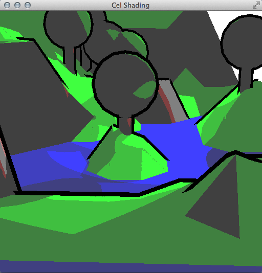
Non-realistic techniques such as cel shading.
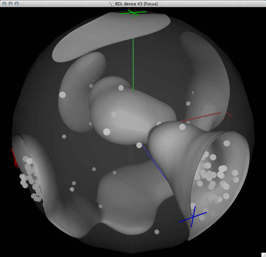
Applications of graphics to scientific visualization. Here I'm plotting iso-density surfaces for a data set consisting of points in SO(3).