2010 January 15 / j d a v i s @ c a r l e t o n . e d u
This tutorial describes how to get started with Python in the Carleton College computer science labs. It is intended to accompany Chapters 1 and 2 of Miller's and Ranum's text Python: Programming in Context. I recommend that you go through all of the sections of the tutorial in order. It is important that you play around some, trying your own variations on the material until you are sure that you understand what's going on. You should come away knowing how to write short programs in Python. You should also know the terms in italics and the answers to the explicit Questions.
In this section we learn how to run the Python interpreter. These instructions are for Mac OS X, which our lab computers use; if sometime you want help running Python on another operating system, just ask.
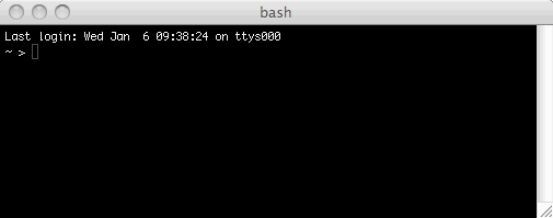
The icon for the Terminal program should already be in your dock; if it isn't, then ask for help. Click on the icon to launch the program. This should bring up a window much like the following, although the color and text may be different.

Put simply, a terminal is a program that lets you run other programs — especially programs with textual interfaces. Right now the terminal is running the program bash. We'll talk more about bash later. The > is a prompt indicating that bash is waiting for your command; your setup may use $ for a prompt instead of >, but that is just a cosmetic difference.
Type python and press the Return key. You have just told bash to run the Python interpreter, which takes over the terminal. bash is still running; it's just temporarily hidden by the Python interpreter.
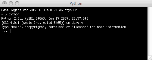
The prompt >>> indicates that the Python interpreter is waiting for your command. Right now, let's not do anything in Python; just press Control-D to exit the Python interpreter. Then you find yourself back in bash; you can quit the Terminal application by pressing Command-Q, if you like.
In this section we use the Python interpreter as a glorified calculator. We also learn how to store values in variables.
Launch the Python interpreter using the directions of the preceding section. Then enter each of the following commands (pressing Return after each one) to see what they do.
3.0 + 6.5
2.2 - 17.2
14.3 * 2.0
14.3 / 2.0
3.0 ** 4.0
Question A: What's wrong with 14.3 * 2.0?
Question B: What does the ** operator do?
When you do long computations on a calculator, it is helpful to store intermediate results in memory. This facility also exists in Python, through the = operator. Try these commands.
x = 5.7
x
3.0 + x
y = x ** 2.0
y
z = x - y
z
z = x + y
z
z = z + 3.0
z
The x, y, and z in the preceding example are called variables. A variable is a named location in the computer's memory. Once you've assigned a value to a variable using =, you can use the value any time you want by simply invoking the variable's name (x, y, or z). You can also assign a new value to a variable at any time.
Question C: Does = have the same meaning in Python as it does in a math class? Does the term variable have the same meaning in Python as it does in a math class?
Question D: What happens when you try to use a variable's value before you've stored a value in that variable? How do you test this?
Variable names are not limited to single letters. Try these commands:
joan = 5.7
joan
timmy_smith = joan ** 2.0
timmy_smith
timmy_smith = timmy_smith + 7.0
timmy_smith
Variable names can be almost any combination of letters, digits, and the underscore _; the only rule is that a variable name cannot begin with a digit. (Also, you should avoid beginning variable names with an underscore, for reasons that we won't explore right now.)
In this section we learn how to import modules and how to find documentation about them.
The Python calculator described in the preceding section is quite limited. For example, it can't compute square roots, it can't do trigonometry, and it doesn't know what π is:
sqrt(16.0)
cos(1.047)
sin(90.0)
pi
Python comes with this functionality installed; it's just not automatically loaded into the interpreter for you to use. The functionality is in the math module. A module is simply a package of Python commands; you load the module using the import command. Then you can refer to any entity within that module using the . operator, as follows.
import math
math.sqrt(16.0)
math.cos(1.047)
math.sin(90.0)
math.pi
Question E: As you may be aware, the sine of 90° is 1; does Python agree?
The math module contains a wide variety of useful functions. You can learn about them in the Python interpreter by entering help(math). This brings up an interactive help viewer in the terminal. You navigate it by pressing the up- and down-arrow keys; you exit it by pressing the Q key. Notice that near the top of the documentation is a URL http://docs.python.org/library/math for a web version of the documentation; you may find the web version more convenient than the terminal version.
Python comes installed with dozens of modules to accomplish various tasks; for example, there are modules for dissecting web pages, for compressing data, and for interacting with the underlying operating system. Here is a complete list of modules that come with Python 2.5.4. You can find hundreds more modules on the web. In this course you will also write your own modules.
Question F: If the math module comes with Python, then why do you have to import it? Why aren't all of these math functions just built into Python? (I'm asking you to speculate here. There are in fact several reasons.)
In this section we learn the distinction between integers and floating-point numbers. The distinction is especially important when we use division. This is our first glimpse of the issue of variable type.
Until now, all of our numbers have had decimal points. But Python can also do arithmetic with whole numbers that don't have decimal points. Try some of these commands for comparison with the ones you used earlier.
7 + 3
7 - 3
7 * 3
7 / 3
7 ** 3
The division example there should have given you pause. To understand what's going on, compare the results of these four commands:
7 / 3
7.0 / 3
7 / 3.0
7.0 / 3.0
In Python (and most other programming languages) there are two types of numbers: integers (whole numbers without decimal points) and floating-point numbers (which have decimal points). For example, the integer 7 and the floating-point number 7.0 are not exactly the same thing in Python. You can see this by comparing the results of 7 / 3 and 7.0 / 3. You can also see it by asking Python what the types the two numbers are:
type(7)
type(7.0)
Question G: When you do an arithmetic operation (+, -, *, /, **) on two numbers of different types, what is the type of the result? Hint: There is a simple rule for this.
Question H: What exactly does the division operator / do on integers? What exactly does the modulus operator % do on integers? Hint: They are related.
Warning: Python 3.0, which the Miller and Ranum text uses, has slightly different conventions for division; it uses / for floating-point division and // for integer division. Let's just use /.
You should be wondering: Why is there a distinction between integers and floating-point numbers? Why isn't there just a single type of number that handles both cases? Which type would that be?
In this section we learn how to write a program in a text editor and run that program in the Python interpreter. The instructions are specific to TextWrangler running on Mac OS X, but other text editors behave similarly. We also learn the most important commands for navigating among folders in bash.
The icon for the TextWrangler program should already be in your dock; if it isn't, then ask for help. Click on the icon to launch the program. You should be greeted with a big, white window.
A text editor is kind of like a word processor (such as Microsoft Word), in that it is a program where you type a bunch of text. However, a text editor lacks the cosmetic features of a word processor, such as fancy formatting of documents. Instead it offers powerful "structural" features, such as the ability to perform sophisticated search-and-replace queries. Loosely speaking, you use a word processor if the document you're typing is going to be read by a human; you use a text editor if the document you're typing is going to be read by a computer. Since Python programs are ultimately read by a computer, we edit them in a text editor.
Type the following commands into the TextWrangler window. In case it's not clear, you're trying to convert a time period measured in seconds into a time period measured in years.
secondsPerYear = 60 * 60 * 24 * 365.25
secondsElapsed = 27000.341
yearsElapsed = secondsElapsed / secondsPerYear
Now press Command-S and save the file to your desktop, giving it a name like secondstoyears.py. The .py suffix is conventional for Python programs, although not strictly necessary.
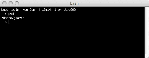
Keeping the TextWrangler window open, also open the Terminal program. Do not launch the Python interpreter in the terminal window; just stay in bash. In bash, first enter the command pwd (followed by Return). pwd means "print working directory"; it tells you where you are in the computer's file system:
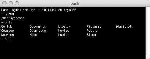
Now use the ls ("list") command to list all of the files and folders here:
Assuming that you saved your secondstoyears.py program to your desktop, now do cd Desktop ("change directory") followed by ls:
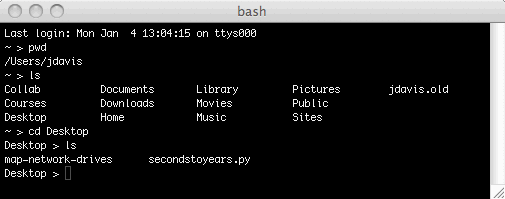
You should see your secondstoyears.py program there. To run the program, enter python secondstoyears.py:
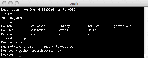
Your program ran, but you didn't ever get to see the answer. This is because you never told the program to produce any output. To fix this, go back to TextWrangler, add the line print yearsElapsed to the end of the program, and save the file. Then return to bash and press the up-arrow key. This takes you back to the last command, which was python secondstoyears.py. Press Return to issue this command again; it should show you the answer:
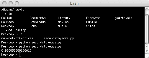
The lesson is this. When you run Python commands in the Python interpreter, the interpreter shows you the result of every command (if there is one). When you type Python commands into a file and run the file, Python does not show you the result of every command; instead, it outputs only what you tell it to, using the print command.
Warning: Python 3.0, which the Miller and Ranum text uses, has slightly different conventions for the print command; it requires parentheses, as in print(yearsElapsed). In Python 2.5.4, which we use, it is better to omit the parentheses.
So there are two ways to interact with Python. The first way we learned was to type individual commands into a Python interpreter running in a terminal. This is useful for when you want to do little experiments, to figure out how a particular Python command works. The second way is to type a sequence of commands into a text file, and then to execute that program in bash using the python command. This is useful when you are writing complicated programs consisting of many commands.
By the way, there is one more useful bash trick to know. If you'd like to go "up" a level, to the parent folder of where you are now, then enter cd ... (That's cd with two dots.) For example, typing this when you're in your desktop folder takes you back to your home folder.
cTurtle and Objects
In this section we practice drawing with the cTurtle module, about which you should have already read in the Miller and Ranum text. We also get our first glimpse of objects.
cTurtle is not installed on your computer, but installing it is easy. Go to the course web page and find the link to cTurtle at the top. Right-click (or control-click) on the link to save the file to your desktop.
A summary of important cTurtle commands is on page 25 of the textbook. An example of how to use these commands is on page 26. Type the example into TextWrangler and save the program to your desktop, with whatever name you like, such as example.py. (The stuff on page 26 is a transcript of someone interacting with Python; there are prompts and outputs there, that you need to strip out.) Then, in the terminal, use ls and cd to navigate to to your desktop, and use python to run the example program.
When you run the program, you should briefly glimpse a window like the one on page 28. Unfortunately, the window immediately vanishes, because the program is finished running. To fix this, add the following line to the program:
raw_input("Press Return to exit.")
Now run the program again. The last line causes the window to stay open until the user presses a key. (The details of how this works aren't important right now.)
Question I: Some of the lines of code listed on page 26 are unnecessary, in that they have no effect on the program's graphical output. Which ones? Strip all of these lines out, and verify that the graphical output is unchanged.
Question J: What is the type of gertrude, according to Python? How would you figure this out in the Python interpreter? How would you figure it out in a Python program? Do it both ways.
There is a substantial amount of jargon in this part of the textbook. Here are the most important bits. First, Turtle is a class, meaning a type of object. The turtle gertrude is an instance or object of that class. (The terms type and class are nearly synonymous; so are instance and object.) All instances of Turtle obey the same commands, such as forward() and right(); these commands are called methods.
We'll learn more about objects later, but here is the big idea. Modern software tends to be huge and complicated. Every day you use software that consists of a million or more lines of code. For the software to work, (almost) every line must be perfect. Furthermore, some parts of the software may use sophisticated mathematics or other technical knowledge that the average programmer doesn't know. Therefore, the people in charge of constructing the software, who may have hundreds of programmers at their disposal, must find an efficient division of labor among those programmers. This is where objects are useful. Each class is a self-contained, manageable chunk of software, that can be written by a single programmer (or a small group). As long as each class behaves according to its agreed-upon specification, the software will work as a whole. Most modern software is constructed according to this strategy, which is called the object-oriented programming style; the software consists of a bunch of objects, of various classes, issuing commands to each other.
Thus far you have been instructed to save files to your desktop. That's okay, but after a while your desktop will get really cluttered. For the long term, I recommend that you make a CS111 folder inside your Documents folder and store everything in subfolders of that folder. Really you can work anywhere you want, as long as you're consistent:
cTurtle, then the program and the module must be in the same folder.
bash, you must use cd to put bash into the correct working directory, where the program is, before executing the program.
cTurtle, then put bash into the correct working directory before launching the Python interpreter.
This section introduces comments, which are a crucial part of any computer program, even though they do no computation.
A comment is a piece of a program, usually a single line, that is ignored by Python. It has no effect on how the program behaves. So what is the point of a comment? You use comments to make little notes that explain how your program works, in plain English.
A comment begins with a hash mark # and runs to the end of the line. For example, here is an excerpt from a typical, well-commented Python program. You don't know the commands used here, and you don't know the point of the code, so you won't understand it. However, you can still appreciate that the comments are trying to explain what the program is doing.
# Prepare the selection system, guessing what the needed capacity might be.
glSelectBuffer(bopagopaSelectionBufferCapacity)
glRenderMode(GL_SELECT)
glInitNames()
# Set an arbitrary selection name, for those users who don't use names.
glPushName(0)
# Let the user draw.
callback()
# End the selection process. This is where overflow may occur.
glFlush()
buffer = glRenderMode(GL_RENDER)
Whenever you write a program in this course, or any other course, or for any job that you do in your entire life, you will comment your code! Furthermore, in each program in this course, one comment is particularly important: At the top of the program there must be a comment containing the name of everyone who contributed to the program.
Why comment code? Because if anyone else ever looks at your code, it will greatly help them understand it. This hypothetical "anyone else" includes you in a few weeks, when you are looking over your old code and no longer remember how it works.
How much commenting should there be? This is trickier; it's a question about the culture of computer programming. It may take you a while to learn how to comment well. Some code is pretty obvious and requires little commenting, while other code is subtle and may need commenting for almost every line. For now, simply put in a comment wherever you think that another student might not understand your thought process. When in doubt, err on the side of too much commenting.
At this point you are ready to tackle Assignment 2: Drawing with cTurtle. Please do so, before continuing.
for Loops and Accumulation
This section describes for loops, which are used to repeat an action a set number of times. We also discuss the accumulator pattern.
A loop is a piece of a program that repeats a sequence of commands over and over again. The sequence of commands that is being repeated is called the body of the loop. There are two kinds of loop in Python: for loops, which repeat the body a predetermined number of times, and while loops, which repeat the body as long as a certain property holds. For now let's just talk about for loops.
Here's a simple example. You can copy and paste this code directly into the Python interpreter, to try it out. (You'll need to press Return a couple of times after pasting.)
for i in range(7):
    print "Hello, world!"
A for loop begins with the keyword for. Next comes a variable called the loop counter, loop variable, or loop index. Here I used i for the loop counter, but there is nothing magical about the name i; you can use any variable name here, such as j, count, or georgeWashington. The in range(7) indicates that the loop body is going to execute seven times. The body simply prints "Hello, world!", so the loop as a whole prints "Hello, world!" seven times. Notice that the body of the loop is indented four spaces; indentation is important in Python, as we'll discuss in a later section.
Usually loops make some nontrivial use of the loop counter. For example, here we print it out on every pass through the loop.
for i in range(7):
    print i
Have you run that code in the interpreter? I hope so. Notice that the loop counter doesn't run from 1 to 7; rather, it runs from 0 to 6 (which is still seven numbers). For a mixture of good reasons and historical reasons, most computer programming languages tend to count from 0. We'll see this again and again — not just in loops.
Now let's get a little more complicated. In the following code, we set up a variable total. (Again, there's nothing magical about that name — I could have called it jenny instead — but total describes what it's going to be used for.) We use the loop to add a bunch of stuff onto total. The body of the loop is two lines long. The two lines are indented the same amount (four spaces).
total = 0
for i in range(7):
    total = total + i
    print total
In the preceding example, the variable total accumulates value as the loop runs. This idea occurs so often in computer programming that it has a name: the accumulator pattern. Python also has a convenient syntax shortcut for accumulation: +=. The following example is identical to the preceding one, except that it uses the += shortcut.
total = 0
for i in range(7):
    total += i
    print total
Now what does this code do?
total = 0
for i in range(7):
    total += i ** 3
    print total
Question K: The two preceding examples produced two different sequences of numbers, but there is a simple mathematical relationship between those sequences. What is it?
The body of a loop can consist of Python code of any kind. In particular, inside the body of a loop there can be another loop; the loops are then said to be nested. On each pass through the outer loop, the inner loop runs its full course. Try this code:
for i in range(6):
    for j in range(6):
        print i + j + 2
I recommend that you make your terminal window at least 36 lines long, because that's how many lines of output there are: six lines printed on each pass through the outer loop. Perhaps the output would be a little clearer if I changed the formatting slightly. The following code does much the same thing, but I'm fiddling with the print commands, so that each pass through the outer loop produces a single line of output with six numbers. Because the code is getting a little tricky, I've added some comments. (For now, don't worry about exactly how these print tricks actually work.)
for i in range(6):
    # Print six sums on a single line.
    for j in range(6):
        print i + j + 2,
    # End that line.
    print
Question L: The numbers here have something to do with dice games. Every player of craps, for example, knows these numbers. So do most introductory statistics students, I expect. Can you figure out what these numbers mean?
In this section we learn how to define our own functions. This is our first example of abstraction.
In Assignment 2 you probably noticed a lot of repetition, where you had multiple chunks of code that did pretty much the same thing. Perhaps you even copied and pasted those chunks, to save typing. Loops, which we discussed in the preceding section, are one way of dealing with repetition; functions are another. For example, suppose that the name of your animal was "CHEETAH". The code for drawing the first "E" would probably be nearly identical to the code for drawing the second "E". In this situation, you want to write a function that draws the letter "E", and then simply invoke that function twice. The same goes for the letter "H".
In computer programming, a function is essentially a sequence of commands with a name attached to them, so that you can invoke the entire sequence of commands by simply invoking the name. A function is a kind of abstraction. Once we have written the function, we (or anyone else) can use the function without worrying about the details of how it works; the details are "abstracted away". Returning to our example, if you had functions to draw each of the letters "C", "H", "E", "T", "A", then your algorithm for drawing "CHEETAH" could be written
Question M: In computing, what is a font? Look it up on Wikipedia if you want. Why am I asking you this right now?
Here is Python code that defines a function to draw the letter "E". The function applies to any turtle. Of course, I have commented the code to help you understand how it works.
def drawE(turtle):
    # Make sure the turtle is pointed to the right.
    turtle.right(turtle.heading())
    # Draw the bottom of the E.
    turtle.down()
    turtle.forward(8)
    # Draw the middle of the E.
    turtle.up()
    turtle.backward(8)
    turtle.left(90)
    turtle.forward(8)
    turtle.right(90)
    turtle.down()
    turtle.forward(8)
    # Draw the top of the E.
    turtle.up()
    turtle.backward(8)
    turtle.left(90)
    turtle.forward(8)
    turtle.right(90)
    turtle.down()
    turtle.forward(8)
    # Draw the vertical line of the E and return to the starting position.
    turtle.up()
    turtle.backward(8)
    turtle.right(90)
    turtle.down()
    turtle.forward(16)
Question N: The line turtle.right(turtle.heading()) makes the turtle point to the right, no matter how it was pointing originally. How exactly does it do this?
To use this function, you create a turtle — let's call it gertrude again — and then you simply call drawE(gertrude). Here is a complete program that draws the letter "E". It is customary to place import commands near the top of the file, so that someone reading the program can see which modules the program requires quickly. It is also customary to put blank lines around a function definition, to ease legibility.
import cTurtle

def drawE(turtle):
    # Make sure the turtle is pointed to the right.
    turtle.right(turtle.heading())
    # Draw the bottom of the E.
    turtle.down()
    turtle.forward(8)
    # Draw the middle of the E.
    turtle.up()
    turtle.backward(8)
    turtle.left(90)
    turtle.forward(8)
    turtle.right(90)
    turtle.down()
    turtle.forward(8)
    # Draw the top of the E.
    turtle.up()
    turtle.backward(8)
    turtle.left(90)
    turtle.forward(8)
    turtle.right(90)
    turtle.down()
    turtle.forward(8)
    # Draw the vertical line of the E and return to the starting position.
    turtle.up()
    turtle.backward(8)
    turtle.right(90)
    turtle.down()
    turtle.forward(16)

gertrude = cTurtle.Turtle()
drawE(gertrude)
raw_input("Press Return to exit.")
At this point you are ready to tackle Assignment 3: Drawing Circles. Please do so, before continuing.
Now let's switch gears a little. Remember earlier in this tutorial, when we were doing stuff like the following?
import math
math.sqrt(16.0)
math.cos(1.047)
Those commands sqrt() and cos() are actually functions defined in the math module. They differ from our drawE() function above in one key way: sqrt() and cos() return answers, whereas drawE() doesn't return an answer. All that drawE() does is draw a little picture; you can't say that drawE(gertrude) is 17 or -31.8, in the same way that sqrt(16.0) is 4 or cos(1.047) is 0.50017107459707022.
To make a function return an answer to you, you have to end that function with a return command. For example, here is a Python function that computes the mathematical function f(x) = x^2 (x squared). Copy and paste this function into the Python interpreter. Then try it out on a few values of x, as in square(3), square(7), etc.
def square(x):
    return x ** 2
For another example, here is a Python function that computes the mathematical function f(x) = x (x + 1) / 2. Try using this function on x = 0, 1, 2, 3, etc. What numbers do you get out? Where have you seen these numbers before?
def myfunction(x):
    return x * (x + 1) / 2
By the way, functions with return values aren't just for doing mathematics; I just started with these in the hope that they might be easily understandable. Later we'll write functions that return all kinds of crazy Python data.
Question O: Earlier I said that drawE() doesn't return an answer. After all, it doesn't even have a return statement. But that is not exactly correct. What is its return value? You won't be able to just figure it out; you have to test it. How?
In this section we learn about True/False values, which are called Booleans. We introduce the logical operators and, or, and not. We use all of these in if statements, which are called conditionals, selections, or branches.
Launch the Python interpreter and try these commands.
5 > 3
3.7 < 3.2
5 + 3 >= 6
5 + 3 <= 10
4.25 + 3.75 == 8.0
12.1 + 14.2 == 26.3
1 != 17 % 3
You see that >, <, >=, <=, ==, and != are operators that operate on numbers, kind of like the arithmetic operators +, -, etc. But whereas the arithmetic operators produce numbers as answers, the comparison operators >, <, etc. produce True and False. True and False are called Boolean values; they are the only Boolean values, in fact.
Most of these operators are easy to understand. In case it wasn't clear, the == operator tests for equality. Note well that the test for equality is not =; this is because = has already been used elsewhere in Python, to assign values to variables. Also, != means "does not equal".
Question P: What was strange about the second equality test above, and why? (A much harder question to ponder: Why wasn't the first equality test also strange?)
Very frequently when we write a computer program, we want the program to do a certain thing in one situation and a different thing in another situation. For example, suppose that we want to write a function that takes in any number and returns its absolute value. The absolute value of a number is how far away from 0 it is on the real number line. For example, the absolute value of 7 is 7, while the absolute value of -4 is 4. In other words, if the number is positive or zero, then it is its absolute value; if the number is negative, then its negative is its absolute value. (Check: The absolute value of -3 is --3, which is 3. Yep.) An algorithm for computing absolute value is then
x as input
x is positive or zero, then output x
x is negative, then output -x
Here is that algorithm, expressed as a Python function absval(), which you can paste into your interpreter:
def absval(x):
    if x >= 0:
        return x
    else:
        return -x
Try it out; it works. The keyword if signals that the flow of the program is about to take one of two paths, depending on the Boolean x >= 0 that comes after the if. If the Boolean is True, then the first indented block of code is executed; if the Boolean is False, then the second indented block is executed.
Here's another mathematical function, constructed using a more complicated conditional. While you read it, keep your eye on the indentations; they indicate which lines are in which parts of the conditional. Does it look familiar, from high school mathematics?
def quadraticSolution(a, b, c):
    discriminant = b ** 2 - 4.0 * a * c
    if discriminant < 0.0:
        return None
    else:
        numerator = -b + math.sqrt(discriminant)
        denominator = 2.0 * a
        return numerator / denominator
Thus far, all of the Python functions we've written have returned either a number or None. But we can also write functions that return Boolean values. Consider
def isEven(n):
    if n % 2 == 0:
        return True
    else:
        return False
Try it out. It works, but it can be simplified a bit. Think about the logic. If n % 2 == 0 is True, then the function returns True; if n % 2 == 0 is False, then the function returns False. In either case, the function returns whatever n % 2 == 0 is. So why not just write the function like this?
def isEven(n):
    return n % 2 == 0
Now let's use our isEven() function for a greater purpose (albeit not much greater, I admit). The following code counts how many even numbers there are between 0 and 99, and prints out the result.
count = 0
for x in range(100):
    if isEven(x):
        count += 1
    else:
        count += 0

print count
The else clause there is rather silly; it adds 0 to the count, which of course has no actual effect. What we really want here is to increment the count if x is even, and do nothing if x is not even. That is, we don't want an else clause at all. This is a common situation in computer programming. Python lets you simply omit the entire else clause:
count = 0
for x in range(100):
    if isEven(x):
        count += 1

print count
By the way, here is yet another version of that code. It's harder to understand than the preceding version; thus I commented it.
count = 0
for x in range(100):
    # Add 1 to count if x is even; add 0 to count if x is odd.
    count += 1 - x % 2

print count
Question Q: Do you think that this version is more or less efficient than the preceding version? Compare the work done in each version.
Sometimes the logic of a program is more complicated than the two branches offered by an if statement. This is no problem, because we can nest conditionals, just as we nested lists above. Suppose that an insurance firm sets automobile insurance prices for students based on their grade point averages. It prefers students with at least a B average; it penalizes students with less than a C average. Then this logic might apply:
if gpa >= 3.0:
    return 350
else:
    if gpa >= 2.0:
        return 375
    else:
        return 450
This situation, in which the else clause of one if statement "cascades" into another if statement, is so common that there is a special syntax for it — elif — that just continues the first if statement. The following code is equivalent; examine the indentations carefully.
if gpa >= 3.0:
    return 350
elif gpa >= 2.0:
    return 375
else:
    return 450
The insurance price code that we just wrote might fit into a larger function that computes the price based on the customer's age, whether the customer is a student or not, and the customer's grade point average, like this:
def price(age, isStudent, gpa):
    if age >= 25:
        return 300
    elif isStudent:
        if gpa >= 3.0:
            return 350
        elif gpa >= 2.0:
            return 375
        else:
            return 450
    else:
        return 400
We need to discuss a few more operators related to Booleans — the logical operators and, or, and not. Describe what each one does, in English.
n = 120
n % 6 == 0 and n % 10 == 0
x = 4.7
x >= 3.0 and x <= 5.5
x = 2.1
not (x >= 3.0 and x <= 5.5)
x = 7
x < 3.0 or x > 5.5
Question R: For the Ares V rocket to take off with a crew (captain, pilot, copilot), all of these conditions must be satisfied:
temp (measured in Celsius) must be above freezing.
rocketIsFueled(), captainIsDrunk(), pilotIsDrunk(), and copilotIsDrunk() that perform as their names indicate. Write a Boolean expression that expresses whether the rocket may launch.
At this point you are ready to tackle the hasWon() part of Assignment 4: Tic Tac Toe.
In this section we learn two new data types: strings and lists. We also practice counting from zero and discuss the issue of mutability.
Thus far in the tutorial we have used three types of data: integers, floating-point numbers, and Booleans. A fourth data type is the string, which is a sequence of (zero or more) characters. A character is a letter, digit, punctuation mark, or any other symbol that is used in text. Spaces, tabs, carriage returns, and other forms of "empty space" in text also count as characters; they are called white space characters.
You usually enter a string in Python by enclosing it in single quotation marks or double quotation marks:
myName = 'Lucy'
myName
type(myName)
yourName = "Leroy Godzilla, Esq."
yourName
You can ask a string for its length like this:
len("Carleton")
There is a + operator for strings. What does it do?
name1 = "Willoughby"
name2 = "McWillowsalot"
name1 + name2
name1 + " " + name2
The following commands extract particular characters from strings.
name = "Joshua"
name[1]
name[2]
name[3]
name[4]
name[5]
How do you extract the first character from a string? What happens if you ask for a character after the last character? How can you use len() and [] together to extract the last character from any string?
The [] operator can be used to extract not just single characters but also entire substrings, as follows.
name = "Shalikashvili"
name[3:7]
name[0:4]
name[:4]
name[4:]
Question S: When you ask for name[3:7], exactly which characters are you getting out of name? Be careful.
You can test whether two strings are equal using the == operator — the same one that tests whether numbers are equal. For example, airport security software might include the following function to give special treatment to people with the names "Osama Bin Laden" and "Big Bird".
def printWarning(name):
    if name == 'Osama Bin Laden':
        print 'This passenger may be wanted by authorities.'
    elif name == 'Big Bird':
        print 'This passenger may be yellow and fluffy.'
    else:
        print 'This passenger is neither worrisome nor delightful.'
Processing text has always been a popular task for computer programs. This is especially true today, now that so much of our computer time is spent on the World Wide Web. As I mentioned on the first day of class (see About CS 111), many web sites are actually programs, written in Python, Perl, or PHP, that spew web pages at your web browser. But what is a web page? It is bunch of text written in a language called HTML. So these web sites are essentially gigantic text-processing programs.
Because text processing is such a common task for Python programs, Python strings come with a wide variety of convenient features, which you access using the . operator. For example:
song_name = "Mississippi Gosh Darn"
song_name.count("iss")
song_name.find("Gosh")
song_name.lower()
song_name.replace("ss", "JOSH")
Question T: What exactly does replace() do? Be careful: What is the value of song_name after you invoke replace()?
Remember when we were using turtles to draw stuff? (I hope so.) We would make a turtle called something like gertrude, and then give the turtle commands such as gertrude.forward(100). Similarly, here we have made a string called song_name and are giving it commands such as song_name.count("iss"). Both turtles and strings are objects, and the commands that they obey are called their methods. You can find a complete list of string methods at Python 2.5.4 String Methods. For now, I'll just show you one more:
song_name = "Mississippi Gosh Darn"
song_name.split()
Although you may intuitively understand what that split() just did, we have just encountered a heretofore unseen feature of Python that deserves explanation: lists.
A list is a sequence of objects of any type: integers, floating-point numbers, Booleans, strings, or anything else in Python. You enter a list using square brackets [ ] and commas, as seen below. Many of the basic operations that we did on strings above also work on lists, in a similar way:
friendList = ["Jane", "Moon Unit", 2.718, "Babatope"]
friendList
type(friendList)
friendList[0]
friendList[1]
friendList[1:2]
len(friendList)
enemyList = ["Daniel Schorr", "Barney Gumble"]
friendList + enemyList
Like strings, lists also enjoy a variety of methods. Here are the most important ones.
friendList = ["Jane", "Moon Unit", 2.718, "Babatope"]
friendList.append("Superman")
friendList
friendList.extend(["Alison", "Elizabeth Bennett"])
friendList
friendList.insert(2, 3.14159)
friendList
friendList.pop()
friendList
friendList[1] = 'Dweezil'
friendList
Question U: For lists, what is the difference between + and extend()?
Question V: Does a string also have the methods append(), extend(), insert(), and pop()? Does a string also let you change the value of the second character using a command such as song_name[1] = 'x'?
Once you've answered Question V, take a moment to review Question T as well. A key concept is lurking around here. Strings are immutable, meaning that they can't be altered. Once you make a string, you can use it to make new strings, but you can't alter that string in place. In contrast, lists are mutable; they can be changed. Python offers another data type called a tuple, which is identical to a list except that it is immutable. Whereas you construct lists using square brackets [ ], you construct tuples using parentheses ( ):
x = (17, 21, 11, "softball")
x[2]
len(x)
type(x)
othertuple = (330, 219)
x + othertuple
# What does this do? Why?
x.append(20)
Question W: Write a function find() that takes two inputs — a list and another object — and finds the index of the object in the list, or returns None if the object is not in the list. For example, if mylist is ['a', 'e', 'frog', 'crepes sussette'], then find(mylist, 'e') returns 1 and find(mylist, 'dog') returns None. Then: What is the difference between your find() function and the built-in Python list method index()? Also, on an unrelated matter, does your find() function work on tuples?
We're almost finished with lists. There's just one more issue to address. What's going on in the following example?
friendList = ["Jane", "Moon Unit", 2.718, "Babatope"]
friendList.extend(["Alison", "Elizabeth Bennett"])
friendList
friendList[4]
friendList = ["Jane", "Moon Unit", 2.718, "Babatope"]
friendList.append(["Alison", "Elizabeth Bennett"])
friendList
friendList[4]
Remember that a list is a sequence of objects of any type. Just as you can put an integer, floating-point number, or string into a list, so you can put a list into a list. The lists are then said to be nested, one inside the other. Nested lists are commonly used to express grids of objects. For example, a Tic Tac Toe board might be constructed like this:
board = [['x', 'o', ' '], [' ', 'x', 'o'], ['o', 'o', 'x']]
board[0]
board[1]
board[2]
len(board)
len(board[0])
board[0][0]
board[0][1]
board[0][2]
board[1][0]
For another example, a spreadsheet written in Python could store some weather data like this:
data = [[None, 'Jan', 'Feb', 'Mar', 'Apr', 'May', 'Jun', 'Jul', 'Aug', 'Sep', 'Oct', 'Nov', 'Dec'], ['Low', -29, -34, -15, 8, 24, 41, 48, 55, 42, 29, 26, -11], ['High', 30, 29, 41, 50, 71, 81, 87, 93, 93, 81, 53, 44]];
data[0]
data[1]
data[2]
len(data)
len(data[0])
At this point you are ready to tackle all of Assignment 4: Tic Tac Toe (assuming that you've read Section 2.6, which explains how to generate random numbers).
while Loops and the Collatz Problem
This section introduces a second kind of Python loop — while loops. It then uses loops and conditionals to investigate a discrete dynamical system called the Collatz problem.
A while loop is kind of a hybrid between a for loop and an if statement. Like a for loop, it loops; however, rather than looping a predetermined number of times, it loops as long as a Boolean is True. Here's a simple example.
i = 0
while i < 7:
    print i
    i += 1
Question X: This while loop is essentially identical to a certain for loop that we discussed earlier. Which one? It turns out that any for loop can be rewritten as an equivalent while loop. How?
Here's another while loop. Try to figure out what it's doing, before reading on.
number = 1
while not (number % 6 == 0 and number % 10 == 0):
    number += 1

print number
The loop is focused on a certain variable number. In fact, the body of the loop increments number and does nothing else. So number starts at 1 and just keeps increasing until the loop terminates. The loop terminates when a certain mathematical condition is satisfied by number — the condition that number be evenly divisible by 6 and evenly divisible by 10. In other words, the code prints the first positive integer that is divisible by both 6 and 10.
Now let's explore a more complicated application of while loops and conditionals. First, paste or type this function into the Python interpreter:
def hotpo(n):
    if n % 2 == 0:
        return n / 2
    else:
        return 3 * n + 1
The function's name hotpo is an acronym for "half or thrice plus one", which describes it pretty well. The function may seem silly at first, but it's actually rather notorious in mathematics. The notoriety arises when we iterate the function. Supose that we start with some value, say 5. We plug this into the function and get 16 as an answer. Then we plug that into the function and get 8. We plug that in and get 4. We plug that in and get 2. We plug that in and get 1. Once we get 1, we stop. Here's some code to carry out the process I just described.
n = 5
print n
while n > 1:
    n = hotpo(n)
    print n
To investigate the behavior of this process for various starting values, let's make a function out of it. We'll name the function after Lothar Collatz, who in 1937 was the first person to study the process.
def collatz(n):
    print n
    while n > 1:
        n = hotpo(n)
        print n
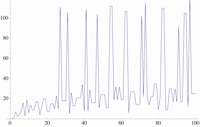
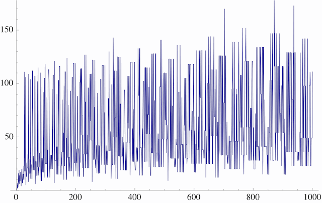
Try this function on various small values of n, such as n = 1, 2, 3, 4, 5, 6, 7. You will find that the number of steps needed for the process to terminate tends to increase as the input value increases, but only vaguely; in fact, the number of steps needed to terminate is fairly erratic. Here's a graph of the phenomenon, for values of n from 1 to 100. On the horizontal axis is n; on the vertical axis is the number of steps required for collatz to terminate when started with that n.
Here's another graph, showing the behavior for values of n from 1 to 1000.
The Collatz system is an example of a discrete dynamical system. Discrete dynamical systems are used throughout the sciences to model situations in which time can be regarded as progressing in discrete steps. Such situations include end-of-day prices on a stock market, year-to-year wildlife populations in a state, and the contents of a computer's memory from one moment to the next. There are also continuous dynamical systems, in which time is continuous; these are typically described by differential equations, and they also have many applications.
Some dynamical systems exhibit a phenomenon called sensitive dependence on initial conditions (SDIC): Small changes in the initial state of the system can have large effects on how the system evolves over time. This is popularly known as the butterfly effect; a butterfly flapping its wings in Brazil creates small air currents, which may affect local winds, which may affect regional weather patterns and, eventually, cause a tornado in Texas. SDIC is one of the key traits exhibited by a chaotic system.
The Collatz system seems to exhibit SDIC, in that small differences in input (say, 26 vs. 27) cause wild differences in the number of steps needed to terminate (10 vs. 111). But SDIC is not what's notorious about this system. Rather, consider the following question: "Does the Collatz system go to 1 eventually for every input? Or is there some input — perhaps some very large number — that causes the Collatz system to spin out of control and never terminate at all?" The answer to this question is not currently known; it is an unsolved problem in mathematics!